May | 2011 | Patterns in Practice

Induction through Failure

May 25, 2011 by Bowen Kerins 2 Comments

I was inspired by a recent post from Ben Blum-Smith about induction to talk about an approach to induction I learned from Al Cuoco. I don’t know its origins, but it really does a nice job of dealing with the issue Ben brings up: you assume you’re right then prove it. But if you’re already right, why prove it?

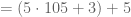
Our curriculum (CME Project Precalculus Investigation 4A, for those playing at home) ties induction to the process of finding closed-form rules to match recursive definitions, such as this one:

$f(n) = f(n-1) + 5, f(0) = 3$

What is $f(23)$ ? All the formula says is that $f(23) = f(22) + 5$ , so that’s no good… except that it is, since now you do the same thing to $f(22)$ , eventually working your way back to the “base case”. This actually works out pretty nicely:

$f(23) = f(22) + 5$

$= [f(21) + 5] + 5$

$= f(20) + 5 + 5 + 5$

$\vdots$

$= f(0) + 5 + 5 + \cdots + 5$

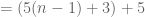
But how many fives? Why is chasing it all the way back to $f(0)$ a good idea? What would change with $f(117)$ ? with $f(n)$ ? This works to find closed-form rules for recursions surprisingly often.

Another way to find $f(23)$ is to count off outputs: $f(1), f(2), \dots$ until you reach 23. More likely, you’ll figure out a pattern to the outputs before you get there… 3, 8, 13, 18…

So now you’ve got these two rules:

$f(n) = f(n-1) + 5, f(0) = 3 \qquad \text{and} \qquad g(n) = 5n + 3$

If I want to prove these two rules will always agree (whenever f is defined, anyway) it’s time for induction. Before that, we really want to be sure the rules agree. This is where technology comes in: using Excel or the TI-Nspire or several other tools, these functions can be entered then compared. (For the Nspire, see page 3 of this document for an example.) Now use the technology to compare $f(23)$ and $g(23)$ … $f(500)$ and $g(500)$ … $f(100000)$ and $g(100000).$

No matter what piece of technology you use, at some point it is going to stop saying that these two functions agree. (On Nspire hardware, this happens somewhere around 100, but depends on the device’s memory.) Say for example that the technology agrees that $f(105) = g(105)$ but $f(106)$ is undefined. How could you show that $f(106) = g(106)$ anyway?

By doing this, the “induction step” process is one that actually happens with a numeric value. So let’s work this one out… evaluating $f(106)$ fails, but we know from its definition that

$f(106) = f(105) + 5$

Oh and we also know that $f(105) = g(105)$ , because the functions agreed up to that point. So:

$f(106) = g(105) + 5$

$= (5 \cdot 105 + 3) + 5$

$= 5 \cdot 106 + 3$

$= g(106)$

The induction step happens naturally, based on the failure of the technology, and based on a numeric example. (Now, try to show that $f(107) = g(107)$ …)

The steps taken above also evolve quickly into a general argument for $f(n)$ simply by using $n$ instead of 106, and noting that 105 should be $(n-1)$ .

$f(n) = f(n-1) + 5$

$= g(n-1) + 5$

$= (5(n-1) + 3) + 5$

$= 5n + 3$

$= g(n)$

And, boom goes the dynamite.

I feel this method does a nice job of dealing with the “proving what you know to be true” issue that surrounds induction. This method can also help with some of the issues around base cases, because it encourages the checking of several cases before trying to complete an inductive proof. Lastly, the extension from the numeric calculation of $f(106)$ to the algebraic calculation of $f(n)$ lines up well with one of Common Core’s mathematical practices, “Look for and express regularity in repeated reasoning“. After all, that’s what induction is all about…

Filed under CME Project Tagged with cme project, induction, Practice #8

Deriving the Quadratic Formula (the easy way)

May 17, 2011 by Kevin Waterman 6 Comments

In Bowen’s post from April 25, he showed a great method for factoring non-monic quadratics. Using that same method, you can derive the quadratic formula pretty cleanly, without lots of fractions, rationalizations, and the like.

The goal is to find a solution to the generic quadratic equation:

$ax^2 + bx + c = 0$

We can’t factor using sums and products, so we resort to completing the square. The equation would be much easier to work with if it were monic. We could divide through by $a$ , but then there’s lots of fractions to keep track of. Instead, let’s multiply both sides by $a$ and make it a quadratic in $ax$ :

$a^2x^2 + abx + ac = 0$

Hmmm. Again, things would be so much easier to complete the square if that middle term were even. We can multiply both sides by 2 to do that, but then the first term isn’t a perfect square. Fine, let’s multiply both sides by 4 then:

$4a^2x^2 + 4abx + 4ac = 0$

Now, just rewrite that a little bit:

$(2ax)^2 + 2b(2ax) + 4ac = 0$

and now we can put our fingers over $2ax$ and see this as a simpler monic:

$F^2 + 2bF + 4ac = 0$

And now, complete the square. First, let’s put that constant on the other side:

$F^2 + 2bF = -4ac$

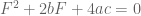
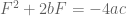
To get a complete square on the left side, we need a $b^2$ , so add it to each side:

$F^2 + 2bF + b^2 = b^2 - 4ac$

The left side is now a perfect square… and the right side looks familiar… Let’s factor the left side:

$(F + b)^2 = b^2 - 4ac$

To solve for $F$ , take the square root of each side:

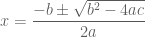
$F + b = \pm\sqrt{b^2 - 4ac}$

and subtract $b$ from each side:

$F = - b \pm \sqrt{b^2 - 4ac}$

What was $F$ again? Lift that finger…oh, yeah, $2ax$ :

$2ax = - b \pm \sqrt{b^2 - 4ac}$

So finish this off by dividing each side by $2a$ :

$x = \dfrac{- b \pm \sqrt{b^2 - 4ac}}{2a}$

And there you have it… the quadratic formula, with no fractions until the final step. Enjoy!

Filed under CME Project

Counting with Polynomials

May 5, 2011 by Al Cuoco 2 Comments

This is to expand on a recent comment I made to “Factoring non-monic quadratics.”

We hear a lot these days about “modeling with mathematics.” One aspect of this is the use of formal calculations as a modeling device. An example, pretty common in many high school programs, is the use of the binomial theorem to compute combinations. So, you can use $(t+h)^{10}$ to compute the number of ways that you can get, say, 4 heads and 6 tails when you toss a fair coins 10 times. Another example is when you use powers of a matrix to get Fibonacci numbers. The calculations not only give you answers, they let you derive properties of the phenomena they model.

One of my favorite uses of formal calculations comes from a project that my daughter gave to her sixth grade class some year ago: compute the most likely sum (and the distribution of sums) when several dice are thrown. For two dice, the problem is fairly standard, and most kids make a 2 by 2 table of all possibilities. For three dice, her students invented all kinds of clever representations, some very algebraic — not in notation, but in spirit. This triggered an idea that has become a recurring theme in our high school program. It goes like this:

If you use expansion boxes to multiply polynomials, you see that the expansion of

$(x+x^2+x^3+x^4+x^5+x^6)^2$

contains exactly the same numbers as the 2-dimensional table that records the possible outcomes when you roll two dice. In other words, the number of ways of rolling a 5 when you throw two dice is the coefficient of $x^5$ in

$(x+x^2+x^3+x^4+x^5+x^6)^2$

It’s the number of ways you can make 5 as a sum of two integers, each between 1 and 6. The same reasoning shows that the coefficient of $x^k$ in

$(x+x^2+x^3+x^4+x^5+x^6)^m$

gives the number of ways you can roll a $k$ when $m$ dice are thrown.

From here, you can use the structure of the expression $(x+x^2+x^3+x^4+x^5+x^6)^m$
to get results about the distribution of sums. For example:

There are $6^m$ possible sums, because this is the sum of the coefficients, and the sum of the coefficients comes from putting $x=1$
There are as many even sums as odd sums (replace $x$ by $-1$ ).
The distribution of sums on three dice whose faces are labeled $\{0, 2, 3, 4, 5, 5\}, \{0, 1, 1, 2, 2, 2\}, \text{and} \{1, 2, 3, 6, 6, 6\}$ can be read off from the coefficients of the product of three different polynomials.
Various factorizations of $(x+x^2+x^3+x^4+x^5+x^6)^m$ give you different information about the distributions. One interesting thing to try is to rearrange the factors of $(x+x^2+x^3+x^4+x^5+x^6)^2$ to try and produce two dice, different from the standard ones, whose distribution is the same as the standard distribution. (This may or may not be possible, we’re not telling.)